38 how to change axis labels in excel 2013

Two-Level Axis Labels (Microsoft Excel) - tips Put your second major group title into cell E1. In cells B2:G2 place your column labels. Select cells B1:D1 and click the Merge and Center tool. (In Excel 2007 the Merge and Center tool is in the Alignment group of the Home tab on the ribbon.) The first major group title should now be centered over the first group of column labels. How to Change the X-Axis in Excel - Alphr Right-click the X-axis in the chart you want to change. That will allow you to edit the X-axis specifically. Then, click on Select Data. Select Edit right below the Horizontal Axis Labels tab....

How to Insert Axis Labels In An Excel Chart | Excelchat We will go to Chart Design and select Add Chart Element Figure 6 - Insert axis labels in Excel In the drop-down menu, we will click on Axis Titles, and subsequently, select Primary vertical Figure 7 - Edit vertical axis labels in Excel Now, we can enter the name we want for the primary vertical axis label.

How to change axis labels in excel 2013

Change axis labels in a chart - support.microsoft.com Right-click the category labels you want to change, and click Select Data. In the Horizontal (Category) Axis Labels box, click Edit. In the Axis label range box, enter the labels you want to use, separated by commas. For example, type Quarter 1,Quarter 2,Quarter 3,Quarter 4. Change the format of text and numbers in labels How to rotate axis labels in chart in Excel? - ExtendOffice 1. Right click at the axis you want to rotate its labels, select Format Axis from the context menu. See screenshot: 2. In the Format Axis dialog, click Alignment tab and go to the Text Layout section to select the direction you need from the list box of Text direction. See screenshot: 3. Close the dialog, then you can see the axis labels are rotated. Rotate axis labels in chart of Excel 2013 How to Add Axis Titles in a Microsoft Excel Chart - How-To Geek Add Axis Titles to a Chart in Excel. Select your chart and then head to the Chart Design tab that displays. Click the Add Chart Element drop-down arrow and move your cursor to Axis Titles. In the pop-out menu, select "Primary Horizontal," "Primary Vertical," or both. If you're using Excel on Windows, you can also use the Chart ...

How to change axis labels in excel 2013. Change axis labels in a chart in Office - support.microsoft.com Right-click the value axis labels you want to format, and then select Format Axis. In the Format Axis pane, select Number . Tip: If you don't see the Number section in the pane, make sure you've selected a value axis (it's usually the vertical axis on the left). Move axis labels from left side of graph to right side of graph Answer LA Lars-Åke Aspelin Replied on July 12, 2010 Right click on the horisontal axis and select Format Axis. In the Format Axis dialogue that appears, click the radio button for "At maximum category" in the "Veritcal axis crosses:" section Hope this helps / Lars-Åke Report abuse 283 people found this reply helpful · Was this reply helpful? Yes No Adjusting the Angle of Axis Labels (Microsoft Excel) - ExcelTips (ribbon) If you are using Excel 2007 or Excel 2010, follow these steps: Right-click the axis labels whose angle you want to adjust. (You can only adjust the angle of all of the labels along an axis, not individual labels.) Excel displays a Context menu. Click the Format Axis option. Excel displays the Format Axis dialog box. (See Figure 1.) Figure 1. The Format Axis dialog box. Using the Custom Angle control, adjust the angle at which you want the axis labels to appear. How to Add Axis Labels in Excel Charts - Step-by-Step (2022) - Spreadsheeto How to add axis titles 1. Left-click the Excel chart. 2. Click the plus button in the upper right corner of the chart. 3. Click Axis Titles to put a checkmark in the axis title checkbox. This will display axis titles. 4. Click the added axis title text box to write your axis label.

How to edit the label of a chart in Excel? - Stack Overflow The latter box will list the "1", "2", etc. numbers that you want to change. Hit the edit button for the right-hand box (Horizontal Category (Axis) Labels), and you will be prompted to enter an axis label range. Instead of selecting a range, though, just enter the labels that you want to see on the x-axis, separated by commas, like so: How to Change Axis Values in Excel | Excelchat To change x axis values to "Store" we should follow several steps: Right-click on the graph and choose Select Data: Figure 2. Select Data on the chart to change axis values Select the Edit button and in the Axis label range select the range in the Store column: Figure 3. Change horizontal axis values Figure 4. Select the new x-axis range How to change chart axis labels' font color and size in Excel? (1) In Excel 2013's Format Axis pane, expand the Number group on the Axis options tab, enter [Blue][<=400]General;[Magenta][>400] Format Code box, and click the Add button. (2) In Excel 2007 and 2010's Format Axis dialog box, click Number in left bar, enter [Blue][<=400]General;[Magenta][>400] into Format Code box, and click the Add button. Easy Ways to Change Axes in Excel: 7 Steps (with Pictures) - wikiHow Steps. 1. Open your project in Excel. If you're in Excel, you can go to File > Open or you can right-click the file in your file browser. 2. Right-click an axis. You can click either the X or Y axis since the menu you'll access will let you change both axes at once. 3.

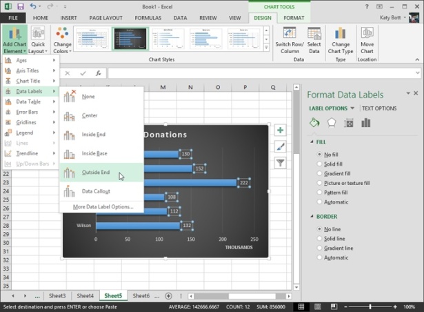
Changing Axis Labels in PowerPoint 2013 for Windows - Indezine Make sure you then deselect everything in the chart, and then carefully right-click on the value axis. Figure 2: Format Axis option selected for the value axis This step opens the Format Axis Task Pane, as shown in Figure 3, below. Make sure that the Axis Options button is selected as shown highlighted in red within Figure 3. Excel Chart Vertical Axis Text Labels • My Online Training Hub Excel 2010: Chart Tools: Layout Tab > Axes > Secondary Vertical Axis > Show default axis Excel 2013: Chart Tools: Design Tab > Add Chart Element > Axes > Secondary Vertical Now your chart should look something like this with an axis on every side: Let's cull some of those axes and format the chart: Click on the top horizontal axis and delete it. How to Add Axis Labels in Excel 2013 - YouTube Axis labels, for the most part, are added immediately to your chart once it is created. in Excel 2013, when the chart is highlighted, you can use the plus sign which is located to the top right of... Custom Axis Labels and Gridlines in an Excel Chart In Excel 2007-2010, go to the Chart Tools > Layout tab > Data Labels > More Data Label Options. In Excel 2013, click the "+" icon to the top right of the chart, click the right arrow next to Data Labels, and choose More Options…. Then in either case, choose the Label Contains option for X Values and the Label Position option for Below.

Analyzing Data with Tables and Charts in Microsoft Excel 2013 | Microsoft Press Store

Excel tutorial: How to customize axis labels Instead you'll need to open up the Select Data window. Here you'll see the horizontal axis labels listed on the right. Click the edit button to access the label range. It's not obvious, but you can type arbitrary labels separated with commas in this field. So I can just enter A through F. When I click OK, the chart is updated.

34 Add Axis Label Excel 2010 - Labels For Your Ideas

How to Switch X and Y Axis in Excel (without changing values) There's a better way than that where you don't need to change any values. First, right-click on either of the axes in the chart and click 'Select Data' from the options. A new window will open. Click 'Edit'. Another window will open where you can exchange the values on both axes.

Chatting about Excel and More: Excel 2016 Charts - X Axis Date Units

How to Add Axis Labels in Microsoft Excel - Appuals.com If you would like to add labels to the axes of a chart in Microsoft Excel 2013 or 2016, you need to: Click anywhere on the chart you want to add axis labels to. Click on the Chart Elements button (represented by a green + sign) next to the upper-right corner of the selected chart. Enable Axis Titles by checking the checkbox located directly ...

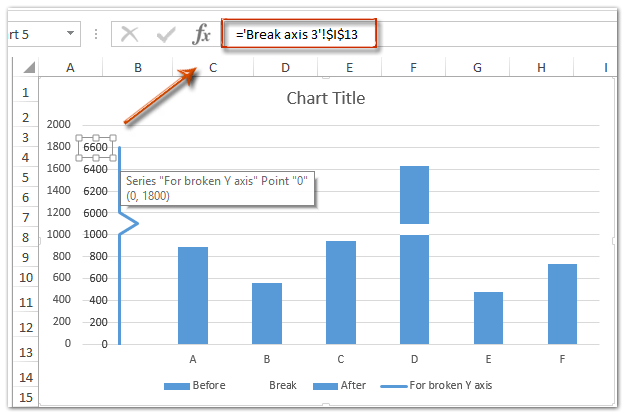
How to break chart axis in Excel?

Format x-axis labels in Excel 2013 - Microsoft Community Using this, you can change the colour of individual months. Key in this article for dummay series is "Use the Below position and Category Names option". The article is for column chart but same can be used for line graphs also. Sincerely yours, Vijay A. Verma @

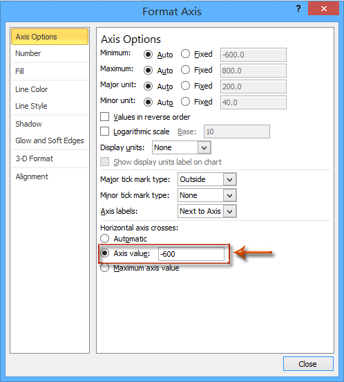
How to move chart X axis below negative values/zero/bottom in Excel?

Changing Axis Tick Marks (Microsoft Excel) - ExcelTips (ribbon) Right-click on the axis whose tick marks you want to change. Excel displays a Context menu for the axis. Choose Format Axis from the Context menu. (If there is no Format Axis choice, then you did not right-click on an axis in step 1.) Excel displays the Format Axis task pane. Make sure the Axis Options tab is selected. (See Figure 1.) Figure 1.

microsoft excel - X axis labels with "super-categories" or "headers" - Super User

How to Label Axes in Excel: 6 Steps (with Pictures) - wikiHow Steps Download Article 1 Open your Excel document. Double-click an Excel document that contains a graph. If you haven't yet created the document, open Excel and click Blank workbook, then create your graph before continuing. 2 Select the graph. Click your graph to select it. 3 Click +. It's to the right of the top-right corner of the graph.

Share :