43 excel chart data labels in millions

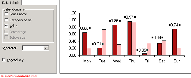
Change the format of data labels in a chart To get there, after adding your data labels, select the data label to format, and then click Chart Elements > Data Labels > More Options. To go to the appropriate area, click one of the four icons ( Fill & Line, Effects, Size & Properties ( Layout & Properties in Outlook or Word), or Label Options) shown here. Excel tutorial: How to use data labels Generally, the easiest way to show data labels to use the chart elements menu. When you check the box, you'll see data labels appear in the chart. If you have more than one data series, you can select a series first, then turn on data labels for that series only. You can even select a single bar, and show just one data label.

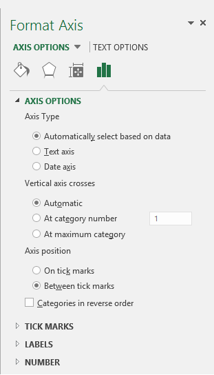
excelunlocked.com › format-chart-axis-in-excelFormat Chart Axis in Excel – Axis Options Dec 14, 2021 · Formatting a Chart Axis in Excel includes many options like Maximum / Minimum Bounds, Major / Minor units, Display units, Tick Marks, Labels, Numerical Format of the axis values, Axis value/text direction, and more. However, there are a lot more formatting options for the chart axis, in this blog, we will be working with the axis options and ...

Excel chart data labels in millions

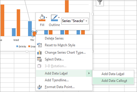
How to Format Number to Millions in Excel (6 Ways) 6 Different Ways to Format Number to Millions in Excel 1. Format Numbers to Millions Using Simple Formula 2. Insert Excel ROUND Function to Format Numbers to Millions 3. Paste Special Feature to Format Number to Millions 4. Using TEXT Function for Excel Number Format into Millions 5. Format Number to Millions with Format Cell Feature 6. Format Chart Numbers as Thousands or Millions - Excel Dashboards VBA To achieve the above simply test for below 1m for thousands and test above 1m for millions. The format for the data label is as follows: [<1000000] 0,K; [>1000000] 0.0,,"m" Choose format label either by right clicking on the series or by pressing Ctrl 1 after you select the series. Tags Chart, label, millions, thousands, Excel Share Edit titles or data labels in a chart - support.microsoft.com The first click selects the data labels for the whole data series, and the second click selects the individual data label. Right-click the data label, and then click Format Data Label or Format Data Labels. Click Label Options if it's not selected, and then select the Reset Label Text check box. Top of Page

Excel chart data labels in millions. Formatting Numeric Data to "Millions" in Excel | AIR Follow These Steps. Select the cell you'd like to format. (A1 in the example) Click the ribbon Home, right-click on the cell, then expand the default to show "Format Cells" dialog. In the Format Cells dialog box, on the Number tab, select Custom, then enter #,, "Million" where it says General. › blog › gantt-chart-excelHow to Create a Simple Gantt Chart in Any Version of Excel Mar 04, 2019 · 11. You can further customize the chart by adding gridlines, labels, and bar colors with the formatting tools in Excel. 12. To add elements to your chart (like axis title, date labels, gridlines, and legends), click the chart area and on the Chart Design tab at the top of the navigation bar. Select Add Chart Element, located on the far left ... Format Number Options for Chart Data Labels in Excel 2011 ... - Indezine Figure 1: Chart with Data Values added as Data Labels. Follow these steps to learn how to format the values used in Data Labels within Excel 2011: Select the chart -- then select the Charts tab which appears on the Ribbon, as shown highlighted in red within Figure 2. Within the Charts tab, click the Edit button (highlighted in blue within ... peltiertech.com › broken-y-axis-inBroken Y Axis in an Excel Chart - Peltier Tech Nov 18, 2011 · For the many people who do want to create a split y-axis chart in Excel see this example. Jon – I know I won’t persuade you, but my reason for wanting a broken y-axis chart was to show 4 data series in a line chart which represented the weight of four people on a diet. One person was significantly heavier than the other three.

Broken Y Axis in an Excel Chart - Peltier Tech 18.11.2011 · For the many people who do want to create a split y-axis chart in Excel see this example. Jon – I know I won’t persuade you, but my reason for wanting a broken y-axis chart was to show 4 data series in a line chart which represented the weight of four people on a diet. One person was significantly heavier than the other three. How do I display millions and billions like this $15M or $10B and still ... You could use a custom cell format for your source data, not sure exactly where you want to break from M to B or how much you want the displayed numbers rounded though. Ex: [>99999999]#.##,,," Cell format to round off to thousands, millions, billions 1. Select the cell or cell range to round off. 2. Do one of the following: Right-click on the selection and choose Format Cells... in the popup menu: On the Home tab, in the Number group, click the dialog box launcher: 3. In the Format Cells dialog box: On the Number tab, in the Category list, select the Custom item. Adding Labels to Column Charts | Online Excel Training | Kubicle To add data labels, just right-click on a data series and click add data labels. To see the data labels clearly, I'll need to select them and change their color to white. The data labels are determined by the vertical axis of your chart. Currently, the vertical axis shows millions, therefore, my data labels are shown in millions as well.

formatting - How to format Microsoft Excel data labels without trailing ... To get this to work, I formatted the cell's of the data column 4 4 4 4 3.5 13.5, by either selecting the column and then right click and format cells or by right clicking on the chart and selecting format data labels.I formatted this with the regular expression $#K so that the data then shows as $4K $4K $4K $4K $4K $14K. The consequence is that the number is rounded to not include the decimal. Data Table to be shown in Thousands - Excel Help Forum Re: Data Table to be shown in Thousands If you are referring to a graph it should be, just click on the graph area, then the data labels to activate them, then right click on them and select format data labels and select the numbers option. (provided I'm not misunderstanding your question.) How to format bar charts in Excel - storytelling with data 12.09.2021 · More Excel how-to’s: To depict a range of values, add a shaded band. To create a frame of reference, embed a vertical line . To show a distribution of data, create a dotplot. For cleaner alignment, put graph elements directly in cells. To have more control over data label formatting, embed labels into your graphs How to format numbers in thousands, million or billions in Excel? Format numbers in thousands, millions, billions based on numbers with Format Cells function If you want to format the numbers in thousands, millions or billions based on the specific numbers instead of only one number format. For example, to display 1,100,000 as 1.1M and110,000 as 110.0K as following screenshot shown. 1.

Charts

How to use Excel Data Model & Relationships » Chandoo.org - Learn Excel ... 01.07.2013 · Things to keep in mind when you using relationships. Same data types in both columns: Columns that you are connecting in both tables should have same data type (ie both numbers or dates or text etc.) One to one or One to many relationships only: Excel 2013 supports only one to many or one to one relationships.That means one of the tables must have no …

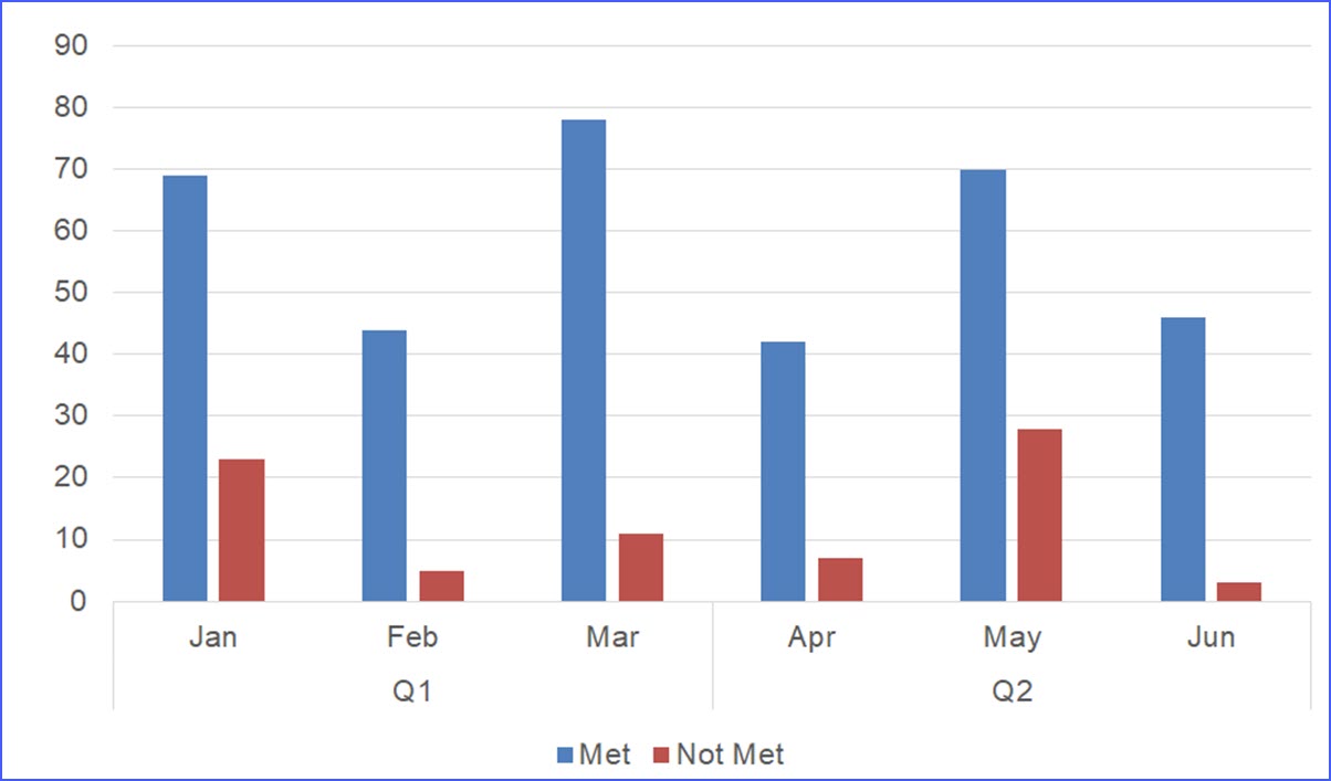
How to Create a Chart with the Axis having Two Categories - ExcelNotes

Display Y Axis Label in Millions or Billions - YouTube If you're dealing with "big" data and charting it, you'd want the labeling to reflect it in words with the shortened numbers. Imagine subjecting your audien...

Chapter 3 Excel 2007/2010 Charts

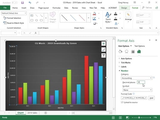
Excel: Display an Axis in Millions - Excel Articles In the resulting settings area, find the Display Units dropdown and choose Millions. Change the axis Display Units. Results: Excel removes the zeros and adds a label indicating that the numbers are in millions. The zeroes are replaced with " Millions" . For more resources for Microsoft Excel Microsoft Excel 2019 VBA and Macros

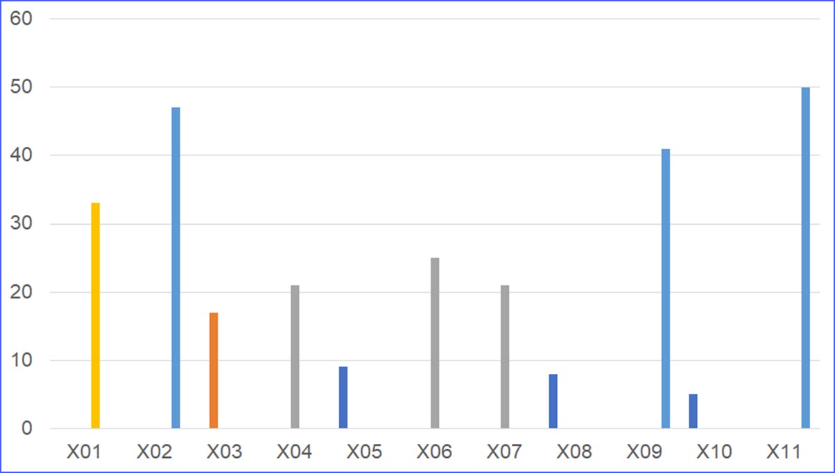
How to Change Bar Chart Color Based on Value - ExcelNotes

Displaying Numbers in Thousands in a Chart in Microsoft Excel To display the numbers in thousands, follow below given steps :-. Select the range B2:B11, and press the key Ctrl+1 on your keyboard. Format Cells dialog box will appear. In the Number Tab, Click on Custom. After clicking on the Custom, related options will get appear.

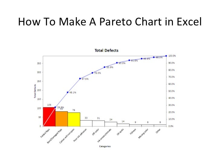
Pareto charts in Excel

Format Numbers to Millions & Thousand in Excel - WallStreetMojo Step #1 - The previous formatting code would show "10 lakhs" as "1000 K," "25 lakhs" as "2500 K," etc. We all know 10 lakh is equal to 1 million. So, we need to format the number in millions instead of in thousands. Below is the code to format the number in millions. Step #2 - Format Code: 0.00,, "Million"

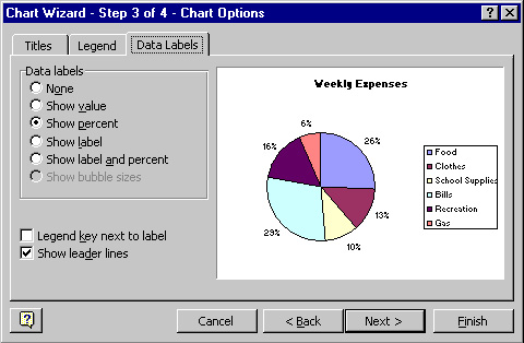
Excel Charts - Chart Options

› en-us › microsoft-365Tips for turning your Excel data into PowerPoint charts ... Aug 21, 2012 · One way to get rid of the gridlines and still provide exact data is to use data labels. In fact, data labels will show your audience the numbers much more clearly. The only trick is to make sure that you don’t have too many numbers on the screen. Here you see the evolution of a chart from grid lines to data labels. Follow these steps: 1.

How-to Use Data Labels from a Range in an Excel Chart - Excel Dashboard Templates

› charts › actual-vs-target-chartActual vs Targets Chart in Excel - Excel Campus Nov 04, 2019 · You can change the order of the data in your chart by choosing Select Data on the Chart Design tab on the Ribbon. Converting a Column Chart to a Bar Chart . Changing your chart to to a bar graph is actually really easy. With the chart selected, go to the Chart Design tab on the Ribbon, and then select Change Chart Type.

Data labels on Excel charts « projectwoman.com

How to format numbers in Excel with millions separators Select the cells you want format. Press Ctrl+1 or right click and choose Format Cells… to open the Format Cells dialog. Go to the Number tab (it is the default tab if you haven't opened before). Select Custom in the Category list. Type in #,##0.0,, "M" to display 1,500,800 as 1.5 M. Click OK to apply formatting.

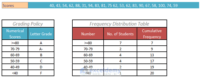
How to Make a Frequency Distribution Table & Graph in Excel?

Tip #1097: Change chart labels on currency values to show in Millions ... Open the desired chart in the Advanced Chart Editor for the XrmToolBox and navigate to the series you would like to change. In the LabelFormat dropdown field, select the desired K, M or B (Thousands, Millions, Billions) formatting. You should also increase the font size at the same time. Remember to click Save and then update the chart. Voila!

Dynamic Number Format for Millions and Thousands - PK: An Excel Expert

Tips for turning your Excel data into PowerPoint charts 21.08.2012 · One way to get rid of the gridlines and still provide exact data is to use data labels. In fact, data labels will show your audience the numbers much more clearly. The only trick is to make sure that you don’t have too many numbers on the screen. Here you see the evolution of a chart from grid lines to data labels. Follow these steps: 1 ...

Excel Format Data Labels In Millions - New Sample v

How to format axis labels as thousands/millions in Excel? Right click at the axis you want to format its labels as thousands/millions, select Format Axisin the context menu. 2. In the Format Axisdialog/pane, click Number tab, then in theCategorylist box, select Custom, and type[>999999] #,,"M";#,"K"into Format Codetext box, and click Addbutton to add it toTypelist. See screenshot: 3.

microsoft excel - Chart fail to interpret dates for label values - Super User

Data Lable in $Millions ($0.0,, "M") and showing percentage label Excel 2003 Posts 2 Data Lable in $Millions ($0.0,, "M") and showing percentage label Hi all, Have a pie chart where I have formated the Value data label to show millions using ($0.0,, "M") number format. EG. 11,796,143 displays as $11.8 M.

Adding rich data labels to charts in Excel 2013 - Microsoft 365 Blog

Actual vs Targets Chart in Excel - Excel Campus 04.11.2019 · So now we have the exact same information, but the data is represented horizontally in a bar chart: More Bar Chart Options. I also wanted to show you that you can add data labels to your chart in order to show: Values Percentage of Target. Learn more about how to go about that from this tutorial. Variance

How To Remove Decimal Places In Excel Graph Axis - Alma Rainer's Addition Worksheets

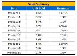
Displaying Large Numbers in K (thousands) or M (millions) in Excel How To Display Numbers in Millions in Excel Right-Click any number you want to convert. Go to Format Cells. In the pop-up window, move to Custom formatting. If you want to show the numbers in Millions, simply change the format from General to 0,,"M" . The figures will now be 23M.

How to Make Excel Charts More Intuitive by Adding Data Labels and Tables - Data Recovery Blog

How to Change the Y Axis in Excel - Alphr 24.04.2022 · Updated April 24, 2022, by Steve Larner, to add details on changing the Y-axis. Working knowledge of Excel is one of the must-have skills for every professional today. It’s a powerful tool that ...

32 How To Label Vertical Axis In Excel - Labels Database 2020

› skip-dates-in-excelSkip Dates in Excel Chart Axis - My Online Training Hub Jan 28, 2015 · An aside: notice how the vertical axis on the column chart starts at zero but the line chart starts at 146?That’s a visualisation rule – column charts must always start at zero because we subconsciously compare the height of the columns and so starting at anything but zero can give a misleading impression, whereas the points in the line chart are compared to the axis scale.

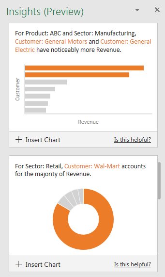
Discover Insights About Your Excel Data - Excel Tips - MrExcel Publishing

› charts › axis-labelsHow to add Axis Labels (X & Y) in Excel & Google Sheets Excel offers several different charts and graphs to show your data. In this example, we are going to show a line graph that shows revenue for a company over a five-year period. In the below example, you can see how essential labels are because in this below graph, the user would have trouble understanding the amount of revenue over this period.

E-xcel Tuts: Add Data Labels to Excel Charts

Skip Dates in Excel Chart Axis - My Online Training Hub 28.01.2015 · In this tutorial we're going to look at how we can skip dates in the Excel chart axis for those dates that have no data. When you plot data in a chart that has a time axis Excel is clever enough to recognise you’re using dates and will automatically arrange the data in date order. The axis will also include all dates in the range, even if you ...

Share :